The Needleman-Wunsch algorithm is a well-known dynamic programming (DP) algorithm used for global sequence alignment. As sequence length increases, the computation time increases significantly. In this blog, we explore the parallelization of this algorithm using anti-diagonal processing, explain its performance, and compare it with the naive approach.
The naive approach to the Needleman-Wunsch algorithm computes the DP table row by row, where each cell is computed sequentially based on the previous one. This approach is simple but very slow for large sequences due to the large number of computations needed and its sequential nature.
On the other hand, the parallel approach breaks the task into independent computations of anti-diagonals. Anti-diagonals are computed in parallel, allowing the workload to be distributed across multiple threads. This significantly reduces runtime for large sequences, though some load imbalance may still occur due to the varying sizes of anti-diagonals.
In the Needleman-Wunsch algorithm, the DP table is computed diagonally, meaning we fill the table along anti-diagonals. Each anti-diagonal corresponds to all pairs of indices (i, j) such that:
i + j = k
Here, k represents the index of the anti-diagonal, and it determines the pairs of indices (i, j) that belong to the same diagonal. The value of k ranges from 1 to n + m, where n is the length of the first sequence and m is the length of the second sequence.
The reason we use anti-diagonals is that they represent independent computations. Each element in an anti-diagonal only depends on values from previous anti-diagonals (those with smaller values of k). Therefore, each element can be computed independently, making it ideal for parallel processing.
The initialization steps for the Needleman-Wunsch algorithm are as follows:
\[ D(0, 0) = 0 \] \[ D(i, 0) = i \quad \text{for} \quad 0 \leq i \leq n \] \[ D(0, j) = j \quad \text{for} \quad 0 \leq j \leq m \]
Where:
After initialization, the recursion relation for filling the DP table for \( i > 0 \) and \( j > 0 \) is as follows:
\[ D(i, j) = \min \left\{ \begin{array}{ll} D(i-1, j-1) + \text{cost}(seq1[i-1], seq2[j-1]), & \text{(Match/Mismatch)} \\ D(i-1, j) + 1, & \text{(Insertion in seq2)} \\ D(i, j-1) + 1, & \text{(Insertion in seq1)} \end{array} \right. \]
Where:
        // Naive Needleman-Wunsch with 2D DP table
        int computeEditDistance2D_naive(const string& seq1, const string& seq2) {
            int n = seq1.size();
            int m = seq2.size();

            // 2D DP table
            vector> dp(n + 1, vector(m + 1, 0));

            // Initialize base cases
            for (int i = 0; i <= n; ++i) dp[i][0] = i;
            for (int j = 0; j <= m; ++j) dp[0][j] = j;

            // Fill the DP table row by row
            for (int i = 1; i <= n; ++i) {
                for (int j = 1; j <= m; ++j) {
                    int match_cost = dp[i - 1][j - 1] + cost(seq1[i - 1], seq2[j - 1]);
                    int gap_seq1 = dp[i - 1][j] + 1; // Gap in seq2
                    int gap_seq2 = dp[i][j - 1] + 1; // Gap in seq1
                    dp[i][j] = min(match_cost, min(gap_seq1, gap_seq2));
                }
            }

            // Return the edit distance (bottom-right corner)
            return dp[n][m];
        }
        // Parallel Needleman-Wunsch with 2D DP table and anti-diagonal strategy
        int computeEditDistance2D_parallel(const string& seq1, const string& seq2, int num_threads) {
            int n = seq1.size();
            int m = seq2.size();

            // 2D DP table
            vector> dp(n + 1, vector(m + 1, 0));

            // Initialize base cases
            #pragma omp parallel for schedule(static) num_threads(num_threads)
            for (int i = 0; i <= n; ++i) dp[i][0] = i;
            #pragma omp parallel for schedule(static) num_threads(num_threads)
            for (int j = 0; j <= m; ++j) dp[0][j] = j;

            // Process each anti-diagonal
            for (int k = 1; k <= n + m - 1; ++k) {
                #pragma omp parallel for num_threads(num_threads) schedule(dynamic)
                for (int i = max(1, k - m + 1); i <= min(k, n); ++i) {
                    int j = k - i + 1;
                    if (j > 0 && j <= m) {
                        // Prefetching to avoid memory latency
                        __builtin_prefetch(&dp[i - 1][j - 1], 0, 1);
                        __builtin_prefetch(&dp[i - 1][j], 0, 1);
                        __builtin_prefetch(&dp[i][j - 1], 0, 1);

                        // Compute DP value
                        int match_cost = dp[i - 1][j - 1] + cost(seq1[i - 1], seq2[j - 1]);
                        int gap_seq1 = dp[i - 1][j] + 1; // Gap in seq2
                        int gap_seq2 = dp[i][j - 1] + 1; // Gap in seq1
                        dp[i][j] = min(match_cost, min(gap_seq1, gap_seq2));
                    }
                }
            }

            // Return the edit distance (bottom-right corner)
            return dp[n][m];
        }
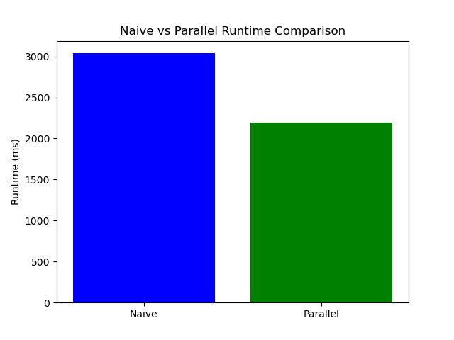
The following results were obtained when running the Needleman-Wunsch algorithm on random sequences of length 40,000:
The following plot summarizes the performance results, illustrating the differences in elapsed times for each method.

The results indicate that the parallelized Needleman-Wunsch algorithm using OpenMP significantly reduces runtime, making it more efficient for large sequences. However, load imbalance due to the varying size of anti-diagonals still presents a challenge. Dynamic scheduling and effective workload balancing are essential for further optimization.
Needleman, Saul B., & Wunsch, Christian D. A general method applicable to the search for similarities in the amino acid sequence of two proteins. Journal of Molecular Biology, 48(3), 443–453. Elsevier BV, 1970. http://dx.doi.org/10.1016/0022-2836(70)90057-4.